Tabular data
Astropy includes a class for representing arbitrary tabular data in astropy.table, called Table. This class can be imported with:
from astropy.table import Table
You may need to also import the Column class, depending on how you are definining your table (see below):
from astropy.table import Table, Column
Documentation
For more information about the features presented below, you can read the astropy.table docs.
Before you proceed
If you have not already done so, download this file and then expand it and go into this directory:
tar xvzf astropy4mpik.tar.gz
cd astropy4mpik
Then start up IPython with the --pylab option to enable easy plotting:
ipython --pylab
Constructing and Manipulating tables
There are a number of ways of constructing tables. One simple way is to start from existing lists or arrays:
>>> from astropy.table import Table
>>> a = [1, 4, 5]
>>> b = [2.0, 5.0, 8.2]
>>> c = ['x', 'y', 'z']
>>> t = Table([a, b, c], names=('a', 'b', 'c'))
There are a few ways to examine the table. You can get detailed information about the table values and column definitions as follows:
>>> t
<Table rows=3 names=('a','b','c')>
array([(1, 2.0, 'x'), (4, 5.0, 'y'), (5, 8.2, 'z')],
      dtype=[('a', '<i8'), ('b', '<f8'), ('c', '|S1')])
If you print the table (either from the noteboook or in a text console session) then a formatted version appears:
>>> print t
  a   b   c
--- --- ---
  1 2.0   x
  4 5.0   y
  5 8.2   z
Now examine some high-level information about the table:
>>> t.colnames
['a', 'b', 'c']

>>> len(t)
3
Access the data by column or row using the same syntax as for Numpy structured arrays:
>>> t['a']       # Column 'a'
<Column name='a' units=None format=None description=None>
array([1, 4, 5])

>>> t['a'][1]    # Row 1 of column 'a'
4

>>> t[1]         # Row obj for with row 1 values
<Row 1 of table
  values=(4, 5.0, 'y')
  dtype=[('a', '<i8'), ('b', '<f8'), ('c', '|S1')]>

>>> t[1]['a']    # Column 'a' of row 1
4
One can retrieve a subset of a table by rows (using a slice) or columns (using column names), where the subset is returned as a new table:
>>> print t[0:2]      # Table object with rows 0 and 1
 a   b   c
--- --- ---
  1 2.0   x
  4 5.0   y

>>> t['a', 'c']  # Table with cols 'a', 'c'
 a   c
--- ---
  1   x
  4   y
  5   z
Modifying table values in place is flexible and works as one would expect:
>>> t['a'] = [-1, -2, -3]       # Set all column values
>>> t['a'][2] = 30              # Set row 2 of column 'a'
>>> t[1] = (8, 9.0, "W")        # Set all row values
>>> t[1]['b'] = -9              # Set column 'b' of row 1
>>> t[0:2]['b'] = 100.0         # Set column 'c' of rows 0 and 1
>>> print t
 a    b    c
--- ----- ---
 -1 100.0   x
  8 100.0   W
 30   8.2   z
Add, remove, and rename columns with the following:
>>> t.add_column(Column(data=[1, 2, 3], name='d')))
>>> t.remove_column('c')
>>> t.rename_column('a', 'A')
>>> t.colnames
['A', 'b', 'd']
Adding a new row of data to the table is as follows:
>>> t.add_row([-8, -9, 10])
>>> len(t)
4
Lastly, one can create a table with support for missing values, for example by setting masked=True:
>>> t = Table([a, b, c], names=('a', 'b', 'c'), masked=True)
>>> t['a'].mask = [True, True, False]
>>> t
<Table rows=3 names=('a','b','c')>
masked_array(data = [(--, 2.0, 'x') (--, 5.0, 'y') (5, 8.2, 'z')],
             mask = [(True, False, False) (True, False, False) (False, False, False)],
       fill_value = (999999, 1e+20, 'N'),
            dtype = [('a', '<i8'), ('b', '<f8'), ('c', '|S1')])

>>> print t
 a   b   c
--- --- ---
 -- 2.0   x
 -- 5.0   y
  5 8.2   z
Finally, every table can have meta-data attached to it via the meta attribute, which can be used like a Python dictionary:
>>> t.meta['creator'] = 'me'
Reading and writing tables
Table objects include read and write methods that can be used to easily read and write the tables to different formats. The tutorial directory contains a file named rosat.vot which is the ROSAT All-Sky Bright Source Catalogue (1RXS) (Voges+ 1999) in the VO Table format.
You can read this in as a Table object by simply doing:
>>> t = Table.read('rosat.vot', format='votable')
(just ignore the warnings, which are due to Vizier not complying with the VO standard). We can see a quick overview of the table with:
>>> print t
     _1RXS        RAJ2000   DEJ2000  PosErr NewFlag   Count    e_Count   HR1  e_HR1  HR2  e_HR2 Extent
---------------- --------- --------- ------ ------- --------- --------- ----- ----- ----- ----- ------
J000000.0-392902   0.00000 -39.48403     19    __..      0.13     0.035  0.69  0.25  0.28  0.24      0
J000007.0+081653   0.02917   8.28153     10    TT..      0.19     0.021  0.89  0.10  0.24  0.13      0
J000010.0-633543   0.04167 -63.59528     11    __..      0.19     0.031 -0.36  0.13 -0.35  0.23     13
J000011.9+052318   0.04958   5.38833      7    __..      0.26     0.026  0.24  0.10  0.00  0.13      0
J000012.6+014621   0.05250   1.77250     11    __..     0.081     0.016  0.05  0.20  0.00  0.26     14
J000013.5+575628   0.05625  57.94125      8    __..      0.12     0.017  0.57  0.12  0.32  0.14      0
J000019.5-261032   0.08125 -26.17556     12    __..      0.12     0.022 -0.26  0.17  0.19  0.29      0
             ...       ...       ...    ...     ...       ...       ...   ...   ...   ...   ...    ...
J235929.2-255851 359.87164 -25.98083     10    _T..      0.23     0.028 -0.43  0.11 -0.30  0.26     13
J235929.3+334329 359.87207  33.72472     11    __..      0.16     0.024 -0.62  0.12 -0.56  0.66     12
J235930.9-401541 359.87875 -40.26139     18    __..      0.13     0.037 -0.73  0.18  0.02  0.82      0
J235940.9-314342 359.92041 -31.72847     19    __..     0.058     0.017  0.17  0.30  0.33  0.34      0
J235941.2+830719 359.92166  83.12195     10    __..     0.066     0.011  0.72  0.14  0.19  0.17      0
J235944.7+220014 359.93625  22.00389     17    __..     0.052     0.015 -0.01  0.27  0.37  0.35      0
J235959.1+083355 359.99625   8.56528     10    __..      0.12     0.018  0.54  0.13  0.10  0.17      9
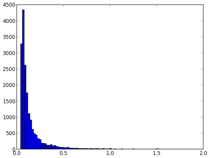
Since we are using IPython with the --pylab option, we can easily make a histogram of the count rates:
>>> plt.hist(t['Count'], range=[0., 2], bins=100)
It is easy to select a subset of the table matching a given criterion:
>>> t_bright = t[t['Count'] > 0.2]
>>> len(t_bright)
3627
Criteria can be combined:
>>> t_sub = t[(t['RAJ2000'] > 230.) & (t['RAJ2000'] < 260.) &
              (t['DEJ2000'] > -60.) & (t['DEJ2000'] < -20)]

>>> len(t_sub)
642
Note about FITS tables
In Astropy 0.2, FITS tables cannot be read/written directly from the Table class. To create a Table object from a FITS table, you can use astropy.io.fits to read in the table to a Numpy array, then initialize the table with it:
>>> from astropy.io import fits
>>> from astropy.table import Table
>>> data = fits.getdata('catalog.fits', 1)
>>> t = Table(data)
and to write out, you can use astropy.io.fits, converting the table to a Numpy array:
>>> fits.writeto('new_catalog.fits', np.array(t))
The main drawback of the current approach is that table metadata like UCDs and other FITS header keywords are lost. Future versions of Astropy will support reading/writing FITS tables directly from the Table class.
Practical Exercises
Level 1
Try and find a way to make a table of the ROSAT point source catalog that contains only the RA, Dec, and count rate. Hint: you can see what methods are available on an object by typing e.g. t. and then pressing <TAB>. You can also find help on a method by typing e.g. t.add_column?.
Click to Show/Hide Solution
>>> t.keep_columns(['RAJ2000', 'DEJ2000', 'Count'])
>>> print t
 RAJ2000   DEJ2000    Count
--------- --------- ---------
  0.00000 -39.48403      0.13
  0.02917   8.28153      0.19
  0.04167 -63.59528      0.19
  0.04958   5.38833      0.26
  0.05250   1.77250     0.081
  0.05625  57.94125      0.12
  0.08125 -26.17556      0.12
      ...       ...       ...
359.87207  33.72472      0.16
359.87875 -40.26139      0.13
359.92041 -31.72847     0.058
359.92166  83.12195     0.066
359.93625  22.00389     0.052
359.99625   8.56528      0.12

Note that you can also do this with::

>>> t_new = t['RAJ2000', 'DEJ2000', 'Count']
>>> print t_new
 RAJ2000   DEJ2000    Count
--------- --------- ---------
  0.00000 -39.48403      0.13
  0.02917   8.28153      0.19
  0.04167 -63.59528      0.19
  0.04958   5.38833      0.26
  0.05250   1.77250     0.081
  0.05625  57.94125      0.12
  0.08125 -26.17556      0.12
      ...       ...       ...
359.87207  33.72472      0.16
359.87875 -40.26139      0.13
359.92041 -31.72847     0.058
359.92166  83.12195     0.066
359.93625  22.00389     0.052
359.99625   8.56528      0.12
Level 2
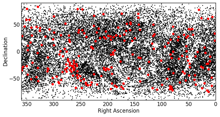
Make an all-sky equatorial plot of the ROSAT sources, with all sources shown in black, and only the sources with a count rate larger than 2. shown in red.
Click to Show/Hide Solution
from astropy.table import Table
from matplotlib import pyplot as plt

t = Table.read('rosat.vot', format='votable')
t_bright = t[t['Count'] > 2.]

fig = plt.figure()
ax = fig.add_subplot(1,1,1, aspect='equal')
ax.scatter(t['RAJ2000'], t['DEJ2000'], s=1, color='black')
ax.scatter(t_bright['RAJ2000'], t_bright['DEJ2000'], color='red')
ax.set_xlim(360., 0.)
ax.set_ylim(-90., 90.)
ax.set_xlabel("Right Ascension")
ax.set_ylabel("Declination")

fig.savefig('tables_level2.png', bbox_inches='tight')
Level 3
Try and write out the ROSAT catalog into a format that you can read into another software package (see here for more details). For example, try and write out the catalog into CSV format, then read it into a spreadsheet software package (e.g. Excel, Google Docs, Numbers, OpenOffice).
Click to Show/Hide Solution
To write out the file:
>>> t.write('rosat2.csv', format='ascii', delimiter=',')
Then you should be able to load it into another software package.
